In this tutorial, I will discuss how to use linear regression with transcriptomic data, in this first part I will introduce linear regression and math behind.

This is the index of the tutorial so you can choose which part interest you

1. Introduction to supervised learning and linear regression
2. Introduction to the dataset and it is preprocessing
3. Digging in the algorithm and the math behind
4. Fit a simple linear regression model
5. Algorithm evaluation: error metrics, assumptions, plots, and solutions
6. Underfitting and overfitting
7. Penalized regression: ridge, lasso, and elastic net
8. Other resources
9. Bibliography

In this first part, I will present the first three chapters, you can skip the math description if you are less interested in mathematical details.

Introduction to supervised learning and linear regression

In the previous tutorials, we have used unsupervised techniques, in this tutorial we will focus on linear classifiers using gene expression data.

For starting, what is supervised learning? Conceptually, imagine you are working on a task and someone is controlling if you are results are correct or not. Similarly, you have a training algorithm and you have labeled data. Each sample (or data observation) of the data set presents a label, which the algorithm has to guess. In the previous tutorial, we did not furnish the label to the algorithm, the clustering algorithms based on the dataset characteristics had to find to which group the samples belong. In unsupervised learning we are not providing labels, we use algorithms to divide into categories (to define a subset, it can be considered as a label). In supervised learning, the algorithm learns on labeled data observation, it is providing an answer and can control on the label if its prediction is correct. As a simple example, if we a dataset of animal images, we will provide the algorithm images which are labeled with the animal’s name. The algorithm will then learn how to discriminate animals and you can use new unseen images to test it is ability.

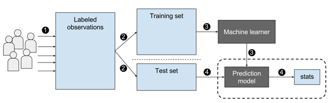
Fig 1. Example of supervised learning. Figure source: here

Conceptually there are two main areas where you use supervised learning:

• Classification: based on the data observations in the dataset your algorithm task is to predict a discrete value (categorical variable). This is the example of the animal dataset we discussed before, you train your algorithm on an image dataset labeled with animals’ species names (categorical variable), and then using new images you ask to predict which animal they represent.
• Regression: the algorithm is predicting the value of a continuous variable. Based on numerous independent variables (a feature of the datasets) the algorithm predicts the variable of the dependent variable. The classical example is you have a dataset with the characteristics of city houses (size, number of rooms, garden extension) and you want to predict the price of the house.

Why this is interesting in medicine and in oncology? Supervised learning can be really useful in diagnosis and outcome prediction (1). An example of classification, machine learning algorithms have been successfully able to classify skin cancer (moles from superficial melanoma, differentiate the different types of skin cancers) (2). On the other hand, predict survival is a regression problem (a particular case, since survival data are censored data). Other tasks where you can use supervised learning are disease relapse, metastasis prediction, treatment option, treatment outcome, and so on.

In general, we can say that machine learning are algorithms (mathematical procedures that describe the relationship between variables, generally an independent variable and many dependent variables). In the case of linear classifiers (or regressors) the topic of this tutorial, the goal is inference (from the collected data, which represents a sample of the population, derives insights on the general population). Linear and logistic regressor are able to make predictions on new data because they make inferences on the relationship between variables. Thus, using these statistical methods we obtain knowledge on the relationship between the dependent and independent variables. As a general example, we have a dataset of some medical parameters (independent variables) and metastasis development (the dependent variable), we can build a linear model to predict on this dataset if new analyzed patients will develop metastasis. The model can also give information on which variables are more associated with the risk to develop metastasis (for instance, size, lymph node involvement). On the other hand, deep learning algorithms are more complex and focus more on accurate prediction (it is more difficult to follow the relationship between variables, also because they take into account nonlinear relationships) and for this reason, they are considered “black box”. These algorithms will be the focus of the following tutorials.

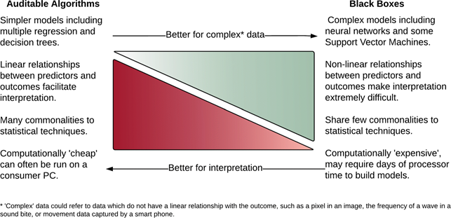
Fig 2. Image source: (1)

In summary, based on the assumption that at least one variable (the dependent) is dependent on other variables, we try to establish a relationship. This is achieved through a function that is mapping the variables to others in a satisfying manner.

As a general terminology:

• Dependent variable: is also called output or response, and for the convention is denoted as y
• Independent variables: also called inputs, predictors, and for convention denoted as x (since normally more than one x1, x2 … xn)

In general, we can say that linear regression is one of the very primitive statistical algorithms, but it is still used a lot. The principle of linear regression will be useful in many contexts and help to understand the more complex algorithms. The algorithm origin is described in the 18th century, there is a discussion about who invented between Carl Friedrich Gauss and Adrien-Marie Legendre, if you are interested you can find more information in the resources at the end of the paper.

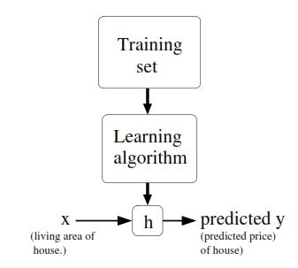
Fig 3 present the concept of a regression problem, if we have a training set with independent variables (X) we can use a function (h) to map X to our dependent variable (y).

We will discuss these points more in details, but for starting we linear models we need:

• Dataset. In our dataset, we have to select which are dependent and independent variables.
• Score function. A function that considers our variables as input and maps to class labels (or the value of a variable in a regression problem). As an example, considering some variables as input vectors, a function f is considering the data points and returns us the predicted class labels.
• Loss function. The loss function is a function that quantifies how good our prediction is (for instance if the predicted class labels are similar to the ground-truth labels, the labels we provided in advance). In regression, the loss function calculates the distance between the predicted value and ground-truth value (the real value of the dependent variable). The higher is the agreement between the prediction and ground-truth labels, the lower is the loss (and this is meaning a higher classification accuracy). The scope is to minimize the loss (meaning increasing the accuracy).
• Weight matrix. Each variable in the input is associated with a weight (how this variable is important for the prediction). Based on the output of the score and loss function, the algorithm is optimizing these parameters (the weight matrix) to increase the accuracy.

There are other parameters, we will discuss them later. The idea is to use an optimization method which minimizes the loss (finding the right set of value for W) in respect of the score function to increase the accuracy.

Introduction to the dataset and it is preprocessing

Let’s start with the dataset. The dataset used in this tutorial is obtained from Warnat-Herresthal et al. (3). They collected and re-analyzed many datasets from leukemia. The dataset and microarray techniques are presented in detail in the previous tutorial.

I write this tutorial in python in Google Colab. As seen in the previous dataset

I have assumed you already have imported the dataset on google drive.

Import necessary libraries and the dataset:

After loading the dataset and necessary library let’s give a glance at the number of available disease conditions in the dataset.

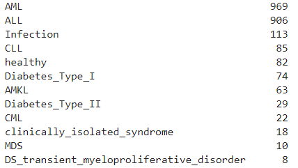
There are two categories that are dominating the dataset: Acute Myeloid Leukemia (AML) and Acute Lymphoid Leukemia (ALL). For easier visualization, we are grouping some categories.

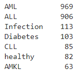
For this tutorial, we will focus only on two cancer types. Then:

and then:

We also filter out the features with low variance and scaling the remaining features.

Digging in the math algorithm

In this section I will describe better the math behind the scene, you can skip this section if you are interested only in how to apply it.

You can find more details in this great tutorial: here?

Linear regression can be defined as a statistical process to estimate an unknown variable (the y) based on some known variables (the x or inputs) if the unknown variable can be calculated using only two operations: scalar multiplication and addition (a linear relationship).

As a start, a linear relationship between hours studied and the percentage score. In this case, the dependent variable is the percentage score (the y) and the hours studied is the independent variable (x). Each data point is a student.

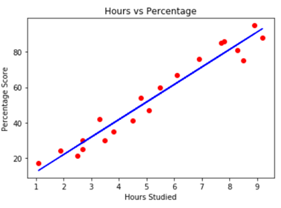
Fig 4. Image source: here

The equation of a straight line is y = mx + b. With m we define the slope of the line and the b is the intercept. Since we have more than one input, we need to change our equation.

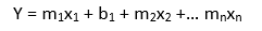
In many cases, m and b are actually indicated as B1 and B0.

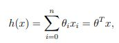
In concept, we are want to estimate our unknown variable (the y) starting from the value of our known variables. As a little notation, X and Y can be real numbers, so we can define this as X=Y=IR. Since we have seen the equation of a straight line we can compute this through the weighted sum of inputs and adding a bias. More formally:

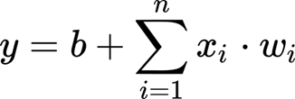
Xi is an input, wi is the weight associated with that input and b is the bias.

To make it a little easier we can consider the bias equal to a variable (the intercept) that has always the same value (equal to 1). For the moment we can simplify the equation.

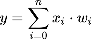
Considering our dataset, we have a matrix of m x n input variables (where m are the number of the observation and n is the number of the features or variables) and we have a vector of dimension n for our dependent variable. We want to transform the last equation in matrix notation (under the hood the algorithm is doing exactly this). Below, we have the weighted sum for a y data point, in simple words is the multiplication of two vectors (the row vector of our input matrix for the column vector that stores the corresponding weights.

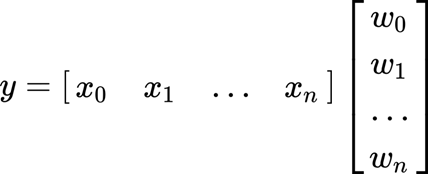
The result is a scalar. If you want to do the calculation for one point, this is the formula.

If we want to the calculation for the whole y variable, you have to multiply a matrix for a vector (will we denote the input matrix as X. y is now a vector, X a matrix, and w is the vector we have seen before.

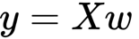
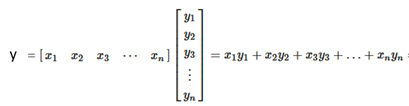
Just to remember as you multiply a matrix for a vector. The product of a matrix (dimension m x n) with a vector (dimension n) is a vector of m dimension. The general formula is:

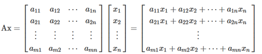
As an example, if we have a matrix A (dimension 2 x 3) and a vector of dimension 3. We first multiply the first row and then the second row. The result is a vector of dimension 2.

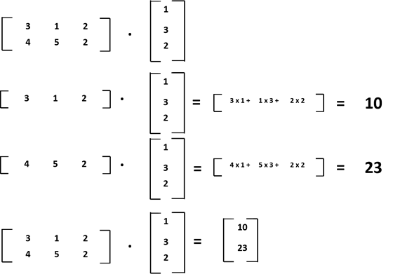
If you think about our dataset, in this case, is how we 2 data point (three input variables) with associated 3 weights and we are calculating the two-point of the y variable.

We know the inputs (these are our dataset variables) now we have to found the weights. The weights are learned from the examples. Generally, we have a training set where we have the inputs (X) and the labeled example (or in regression the corresponding value of the dependent variable y). Based on this, we use the values of x and y to calculate w.

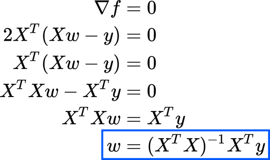
In the simplest form, we can derive from the precedent equation by simple solving for w.

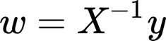
There is to do an assumption, the number of data points has to be at least one more the number of inputs (so, let’s say we have 4 inputs variables we need at least 5 observations). This is a regression line (technically is a regression line only when n inputs are equal to one, for 2 is a plane, for 3 a 3-d plane, and so on).

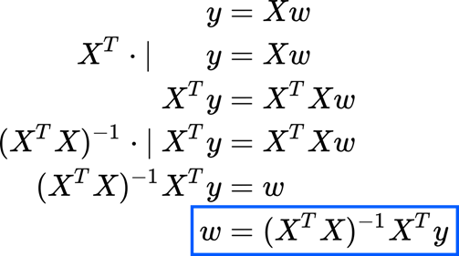
This equation actually is for an ideal case. Most of the time, our data points are not fitting a perfect line (as an example in Fig 3, the data points are not perfectly on the line, like there is some random noise around our regression line). This meaning we cannot find an exact solution for w, then the aim is to find the best solution for our weights. If the equation has no solution, technically y is not belonging to the column space of X. So, instead of using y, we will use its projection on the X column space. How we can do this? We start multiplying the transpose of X to both sides of the equation and then solve the equation.

To understand the matrix transposition, you can find in the figure some examples:

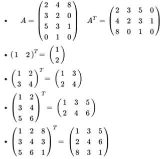
As a general rule, if you want to calculate the transpose of the matrix, you image a diagonal axis starting from the first point on the left to the bottom (the last on right) and then you reflect the matrix (the imaginary line is the symmetry axis). Alternatively, you rotate the matrix clockwise (90 degrees) then you start to exchange the rows like the first with the last and so on (looking at the first matrix in the figure, you exchange the first and third, while the second remain in position).

About the inverse of a matrix, A -> A-1. Here an example for a matrix of dimension 2x2, for different matrix dimension is much more complicated to calculate and there are many different methods, if you are interested to dig you can read these articles: here and here

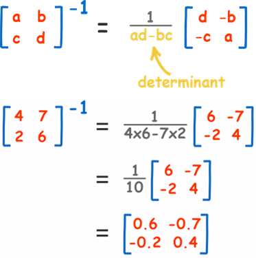
Fig 6. Adapted from: here

Calculus approach

There is another approach you can follow to find w and this is calculus. We will discuss this briefly. we discussed before the idea of an error function. In this case, what we are doing is to define an error function and use calculus to find the weights that minimize our function. Let’s step back to better understand. In the easiest case, we have just one input variable and one dependent variable. As we said before, there is no perfect correspondence between our line and the data points. In practice, we have a function:

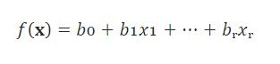
that calculate the dependencies between the inputs and outputs. With this function, we estimate for each input the output. For each observation, we can calculate the correspondence between our prediction and the ground-truth value:

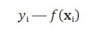
This difference is called the residual. The idea is to find the best weight to reduce the residuals to the smallest value. In general, to find the best weight in this scenario you use the method of ordinary least squares, you minimize the sum of the squared residuals (SSR) with the formula

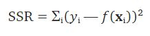
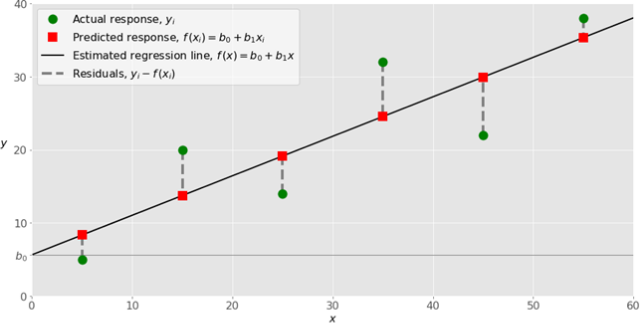
Fig 7. Figure source: here

This is the simplest case, but here we have an input matrix. The function here is doing exactly the same, it takes into account the difference between each true y and our y estimation (the one obtained by the regression model). Then these differences are squared and all summed. This we can write in matrix notation as:

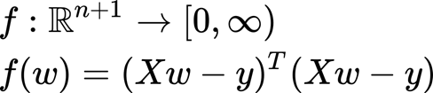
In the same view, the idea is to find a minimum of this function (this should be where the gradient is zero). We will discuss the equation briefly but if you have interest in the process you can find additional details here.

this is for computing the gradient:

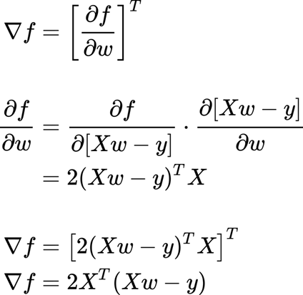
Then we need solving for w (after all, we are interested in the weights). So we set equal to zero.

As you see this solution is the same, we found a linear algebra approach. This is meaning that minimizes the sum of squared errors and projecting y on the column space of X are giving the same result. This solution is telling as that to have a solution the matrix has to be invertible. This requirement is generally met when we have more observations than input variables.

We have found a critical point, but we do not know if this point is the minimum or the maximum point of the function. How we can know it? We have to compute the Hessian matrix to establish the convexity or concavity of the function. The Hessian matrix basically describes the local curvature of a function of many variables. You can find more information here.

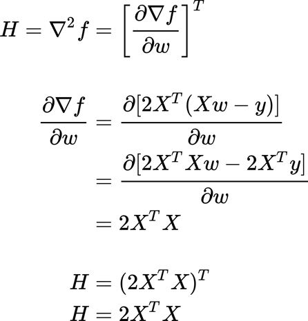
We will multiply for a vector z (of real values).

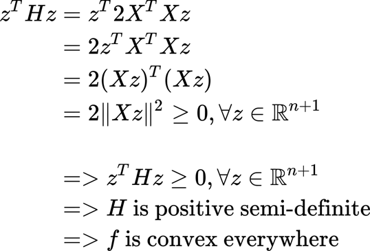
What is important to retain here is that our function is convex, so the solution for w is a minimum point of the function (which is what we were looking for).

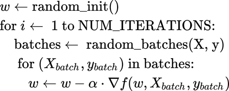
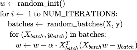
Stochastic Gradient Descent (SGD)

Behind the hood, scikit-learn is using the ordinary least squares method. However, when you are using a penalty term is using stochastic gradient descent (SGD). Since we will discuss penalty, we will discuss briefly SGD (we will go in deep on SGD in other tutorials since it has more sense to discuss in detail when facing neural networks). To discuss briefly we would say that SGD is a powerful algorithm and critical in optimization for many machine learning techniques.

To recapitulate quickly, since we are learning from examples, we have a training set (with input variable X and dependent variable y) and we want to find a function h that h(xi) is a good predictor for the corresponding yi. If we are planning to estimate the y as a linear function of x:

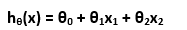
Theta is just another notation for our weight, and we rewrite this equation as we have seen before:

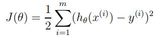
And from here we can calculate a cost function J, as we said before the main idea is to compute a function that determines how close a h(xi) is to yi. One of the main reasons we use square error is because is easier to solve (the derivative is a linear function, so it easy to solve):

Now we will use gradient descent to minimize this function. In simple word, gradient descent starts with an initial weight (theta) and it repeatedly updates it. The update is for all the values of J since we have different weights.

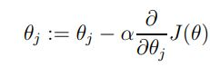
This is updated by a certain quantity defined before which is called learning rate (a). The algorithm takes this step (of dimension a) and iteratively changing the weight (theta) to converge to a value that minimizes J. the algorithm takes a step in the direction of the steepest decrease of J. This can be represented as:

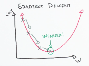
Fig 8. Figure source: here

For a single training example this is the update rule:

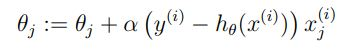
Which more generally is (you have to use the partial derivative):

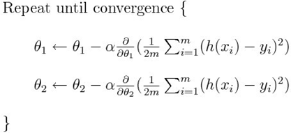
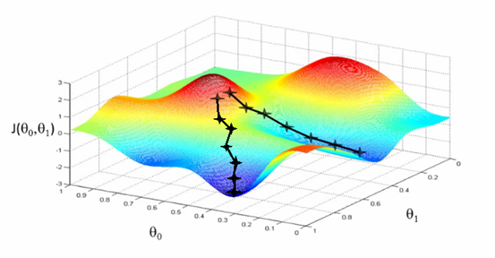
Fig 9. Figure source: here

What we can understand from the equation and the figure above, SGD is practically updating the parameters multiplying the partial derivative of the difference between an estimated value ( h(x)) and the true value (y), multiplying it for a (learning rate). In concrete, the derivative in simple words is driving the update of the parameter toward the minimum (is giving the direction of change) while the learning rate is specifying how much you have to change the value of the parameter.

For further detail on SGD: here?

In our context:

Remember a is the learning rate, we will discuss later in detail. Computing the gradient:

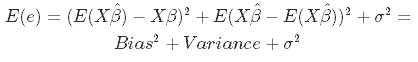
Bias-Variance trade-off

The last point to discuss is the Bias-Variance trade-off. Let’s start with this equation:

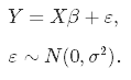
This equation shows that if you want to predict y, this is a combination of X (multiplied for a weight) plus a normally distributed error term that has a variance a^2.

Then as we said we minimize a loss function to obtain the estimated weights B-hat (which is a little different from the true B).

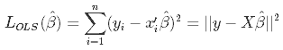
Which in turn using the ordinary least square (OLS) method is:

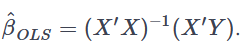
So far nothing new. The bias is the difference between the true population parameter and the expected estimator. It basically measures the accuracy of estimates. E is standing for expectations.

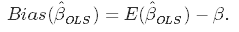
While variance measures the spread (called also the uncertainty)

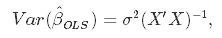
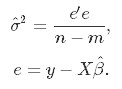
And we can estimate the variance from the residuals:

If you want more details on these calculations: here

A simple way to understand what these terms are is by looking at the bull’s-eye image. The bull’s-eye is the true population and we want to estimate ?, the shoots are the value of our estimates (in this case 4 different estimators).

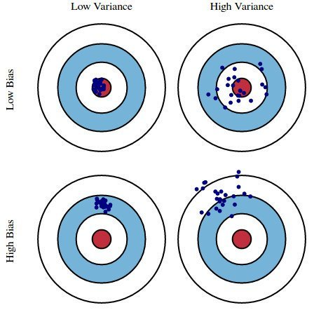
Fig 10. figure source from: here?

We desire that both variance and bias are low, high values lead to poor prediction. Indeed, the model error is composed of 3 parts: the bias, the variance, and the unexplainable part.

Specifically, in OLS the problem is the variance, due to too many predictor variables highly correlated among them and also depending by the number of inputs (if m is approaching n, the variance is close to infinity).

Generally, the solution is to reducing variance at cost of introducing some bias. This is the principle of regularization (which will be discussed in the next part of this tutorial). The next figure is summarizing this point. The concept is that increasing the number of inputs is creating complexity and the variance increase. At the same time the bias decrease. At the right point, we have the simple linear regression. So, the idea is to reach the optimal point.

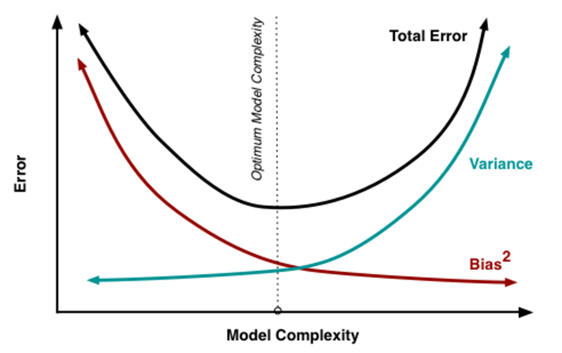
Fig 11. figure source from: here